In Proceedings of the IEEE/RSJ International Conference on Intelligent Robots and Systems (IROS'06), Pages 2711-2716, Beijing, China, October 2006.

Sounds Good: Simulation and Evaluation of Audio Communication for Multi-Robot Exploration

Pooya Karimian         Richard Vaughan         Sarah Brown
Autonomy Lab, School of Computing Science, Faculty of Applied Sciences
Simon Fraser University, Burnaby, BC V5A 1S6, Canada
Email: [pkarimia,vaughan,sbrown1]@cs.sfu.ca

Abstract

In order to guide the design of a new multi-robot system, we seek to evaluate two different designs of audio direction sensor. We have implemented a simple but useful audio propagation simulator as an extension to the Stage multi-robot simulator. We use the simulator to evaluate the use of audio signals to improve the performance of a team of robots at a prototypical search task. The results indicate that, for this task, (i) audio can significantly improve team performance, and (ii) binary discrimination of the direction of a sound source (left/right) performs no worse than high-resolution direction information. This result suggests that a simple two-microphone audio system will be useful for our real robots, without advanced signal processing to find sound direction.

1  Introduction

Numerous types of sensors and emitters have been used in robots. Audio (defined as sound signals at human-audible frequencies) is occasionally used, but is by no means as popular as the cameras and range finders fitted to most mobile robots. In contrast, we observe that audio signaling is extensively exploited by animals. The most obvious example is human speech communication, but many non-human mammals, birds and insects also use sound in spectacular ways. Of particular interest to the multi-robot systems builder is the use of audio signals to organize the behavior of multi-agent systems, for example by sounding alarm calls or establishing territories. In robots, audio is used both for passively sensing the environment and as a means of communication. Buzzers and beepers are common debugging tools, allowing humans to perceive aspects of a robot's internal state over several meters and without line-of-sight. Some systems, including research robots and toys, have speech synthesizers to make human-understandable sounds. Conversely, speech recognition systems have been employed for robot control by humans. But the use of audio as a robot-to-robot communication medium is not well studied. The most common means of communication between robots is through wireless data links which have the advantages of being robust, fast and relatively long range. Line-of-sight communication systems are also used, usually implemented using infrared signaling and the IRDA protocol. However, there are some interesting properties of sound which may make it attractive as an alternative or complementary medium for robot-robot communication. First, unlike light- or infrared-based systems, audio signals do not need line of sight. Audio is propagated around obstacles by diffraction and by reflection from surfaces. However, reflected audio signals may be greatly attenuated as their energy is partially absorbed by the reflecting material. Audio signals are typically affected by robot-scale obstacles much more strongly than are radio signals. The strong interaction between audio and the robot-traversable environment means that useful environmental information can be obtained from a received audio signal in addition to information encoded into the signal by its producer. This insight can be seen to motivate previous work using audio in robots. For example, robots can follow an intensity gradient to find a sound source. In many environments, such as an office building, the intensity gradient closely follows the traversable space for a robot. Further, the steepest intensity gradient generally takes the shortest path from source to the robot. Huang [1] showed sound-based servoing for mobile robots to localize a sound source. Østergaard [2] showed that even with a single microphone, an audio alarm signal has a detectable gradient which can be used to track down the path toward the sound source and they used the audio signals to help solve a multiple-robot-multiple-task allocation problem. Animals, including humans, have the ability to identify the 3D direction of sound source (with some limitations). A mechanism that performs this task with amazing precision has been extensively studied in owls [3]. Several authors, e.g. [4], have demonstrated artificial sensor systems that can accurately localize sound sources. Our interest is in designing systems of many small, low-cost robots, each with relatively little computational power and memory. Microphones are attractively low-cost, and we aim to leverage the power of these sensors as demonstrated by their use in animals. We desire to keep our robots as simple as possible, to allow us to examine minimal solutions to robotics problems. The question that motivated the work in this paper is simple: do our robots need accurate sound localization to get significant benefits from audio signaling?

2  Tools and Task Definition

In addition to microphones, our robots are equipped with some other low-cost sensors: a single loudspeaker, infrared rangers, and a low-resolution CCD camera with the ability to detect two different color markers. The world is large compared to the size of the robots, and accurate global localization is not feasible. To guide the design of the real robots we model these sensors in the Player/Stage [5] robot interface and simulation system. At the time of writing the standard Stage distribution does not simulate audio communication between robots, so we extend Stage with an audio propagation model. The model makes the simplifying assumption that sounds traverse the shortest path from speaker to microphone and the received signal intensity is a function only of the length of the traversed path. Audio may be useful in many practical robot applications. As a motivating example, we examine a general resource-transportation task which requires robots to explore the world to find the (initially unknown) location of a source and sink of resources, and then to move between the source (loading) and the sink (unloading) locations. The metric of success is the time taken for the entire team to complete a fixed number of trips between the source and the sink. The importance of this task is that it is functionally similar to various exploration and transportation scenarios and it has been previously studied (e.g. [6]). The robots are individually autonomous and do not have a shared memory or map. The source and sink locations are initially unknown and the robots must find them by exploring the environment. It is straightforward to implement a robot that can perform this task with these constraints. The amount of work done - measured by the total number of source-to-sink traverses per unit time - can be increased by adding additional robots. If the robots act independently, performance increases linearly with the number of robots added until interference between robots becomes significant [7]. If the robots are not independent, but instead actively cooperate by sharing information, we can expect to improve performance further. In these experiments we examine the effects on overall system performance when robots generate audio signals to announce the proximity of a target. On hearing an audio signal, a robot can head in the direction from which the signal was received, and thus reduce the time it takes to find a target. We expect that the robots can reach more targets if they signal to each other in this way, and indeed our results show this effect. The more interesting experiment is to severely restrict the robot's ability to detect sound direction. We examine the difference in performance between robots that can determine the direction of a sound source with perfect accuracy, and those that can tell only if the sound was louder at the front or rear microphone: 1 bit of direction information. The 1-bit system is significantly easier and less computationally costly to implement, so it is useful to see how it performs compared to an idealized perfectly accurate direction sensor.

3  Audio Model

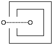
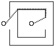
Figure 1: The shortest-path audio model models the large difference in received signal intensity in the scenarios depicted in (a) and (b). In this figure, solid lines are walls, circles are the sender and receiver robots locations and dotted lines are shortest audio paths. Audio propagation in an office-like environment is very complex. Sound waves are partially reflected, partially absorbed and partially transmitted by every material with which they interact. Different materials interact with the signal in frequency- and amplitude-dependent ways. Physically accurate modeling is very challenging. We take a pragmatic approach similar to those used in computer games where the simulation needs to be realistic enough to be useful, while being computationally feasible to run at approximately real-time [8]. Our model models the sound propagation by the shortest-path from speaker to microphone only. Reflections or multiple paths are not modeled and audio is not transmitted through solid walls. This simple model is sufficient to exhibit some of the useful features of the real audio transmission, such as the locality and directionality of sound and the existence of local environmental gradients. For example the shortest-path audio model models the large difference in received signal intensity in the scenarios depicted in Fig. III and Fig. III. To compute the shortest-path from sound source to sound sensor without passing through walls, a visibility graph is generated [9] [10]:

For a map M in which obstacles are defined as a set of polygonal obstacles S, the nodes of visibility graph are the vertices of S, and there is an edge, called a visibility edge, between vertices v and w if these vertices are mutually visible.

To find the shortest-path between two points, these points are added as new nodes to the visibility graph and the visibility edges between these new nodes and the old nodes are added respectively. The value of each edge is set to the Euclidean distance between its two nodes. Then by running the Dijkstra [11] algorithm from the source to the destination the shortest distance and shortest-path between these two nodes is found.

4  System

4.1  Robot Platform Requirements

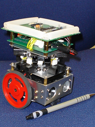Figure 2: Prototype of Chatterbox, a small robot, running Linux and equipped with different types of sensors and emitters. These experiments are run in simulation using Player/Stage, in order to guide the design of a group of real robots. Our Chatterbox project is building 40 small robots to study long-duration autonomous robot systems. The robots run Player on Linux on Gumstix single-board computers. They will work in large, office-like environments: too large for the robot to store a complete world map. The simulations use only sensing and actuation that will be available on the real robots. Robot controllers are written as clients to the Player robot server, which provides a device-independent abstraction layer over robot hardware. Stage provides simulated robot hardware to Player by modeling the robots' movements and interactions with obstacles, and generating appropriate sensor data.

4.2  Audio Model Implementation

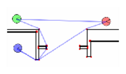
Figure 3: An example of a bitmap and a set of refraction points. These three robots are sending audio signals and the lines show the calculated shortest audio paths. The proposed audio simulator is a Player client, based on Gerkey's Playernav utility (included with the Player distribution). The audio client obtains map and robot position data from Player, and acts as a communication proxy between robots. Robots emit "sound" by making a request to the audio client. Our audio model client calculates the shortest distance between the transmitting robot and all receiving robots. The intensity of the received signal is determined by the distance traveled. If any of the robots receive a sound above a minimum threshold, the audio client transfers the sound data including received intensity and direction to the receiving robot. Our audio propagation model requires that obstacles be defined as a set of polygons but the Player map interface provides obstacle maps in a bitmap format. In order to convert the bitmap to a format that can be used to generate a visibility graph quickly, a 3 ×3 mask is used to find obstacle corners. By scanning this 3 ×3 mask some points are labeled as refraction points, the points at which audio can change direction. Fig. 3 shows an example of a set of refraction points and the audio path found by this method.

4.3  Exploration

Two arbitrary, distinct world locations are defined as the source and the sink, respectively, of resources for our transportation task. The locations are marked with optical fiducials (hereafter markers), visible in the on-board camera only over short distances with line-of-sight. Robots must find the source and sink locations and travel between them as quickly as possible. Without global localization, the robots need to explore the world to find the markers that indicate source and sink. On reaching a marker, a robot stops there for a short, fixed amount of time intended to model the robot doing some work at that location, such as grasping an object. After this time is up, the robot seeks the other location marker. This way of implementing the system permits marker locations to change arbitrarily over time. There are many different approaches that can be taken for exploration to find markers. One suitable method is frontier-based searching proposed by Yamauchi [12], in which each robot uses an occupancy grid with three states: empty, obstacle, and unknown/unexplored for each cell to store the global map. At the start, the entire world is unexplored, but as the robot moves, the occupancy grid will be filled using the sensor readings. Frontiers in this occupancy grid are defined as those empty cells that have an unknown cell in their 8-connected neighborhood. Each robot moves towards the nearest frontier and gradually it explores all the traversable areas with a greedy strategy to minimize the traveling cost. The exploration is complete when there are no more accessible frontiers. The frontier-based approach guaranties that the whole traversable area of the map will be explored. We use an adaptation of this approach described below.

4.4  Path Planning in a Local Map

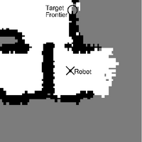
Figure 4: (a) Local map: an occupancy grid built by a robot over a period of time. In this image, white shows empty area, black shows known obstacles (enlarged by the robot size), and gray shows unknown area. (b) Traversibility map: the darker the cell color, the harder going to that cell is (c) Potential field map: robot can follow the gradient to reach the target. Our constraints require that the robot has no a priori global map, has no means to globally localize itself, and has conventional odometry with unbounded error growth. We wish to avoid the memory and computational cost of producing a global map, yet still perform effective exploration. Our approach is to maintain a short-range occupancy grid of robot's current neighborhood, centered at the robot. We call this occupancy grid a local map. As the robot moves, the local map is updated continuously from sensor data. Information may "fall off" the edge of the local map as the robot moves, and is lost. Figure IV-D is an example of a local map built by one robot over a period of time, in which white, black and grey cells indicate empty, obstacle, and unknown areas respectively. To explore the world, we use frontier-based exploration, where the state of all cells outside the map is assumed to be unknown. This means that all empty cells on the map border are frontiers. We modify the original frontier-based method so that each cell value in the map expires after a fixed amount of time and reverts to unknown. This is to cope with the dynamic elements of the world such as other robots, which may look like obstacles to the sensors. For obstacle avoidance and planning we combine the local map with a potential field path-planning method due to Batavia [13]. Using the collected environment information stored in the local map, first a traversibility map is built. The traversibility map is the result of applying a distance transform to the obstacles in the local map. The distance transform operator numbers each cell with its distance from the nearest obstacle, so a non-empty cell is numbered as zero; all its empty neighbors will be one and so on. In our implementation, a city-block ("Manhattan") distance metric is used, thus assuming travel is only possible parallel to the X and Y axes. Figure IV-D shows an example local occupancy-grid map and Figure IV-D shows the corresponding traversibility map. Occupancy grid cells marked "unknown" are handled as empty cells. An exponential function on the value of a cell in traversibility map shows the cost of moving to that cell. This forces the robot to maintain a suitable distance from obstacles while not totally blocking narrow corridors and doorways. A wave-front transform is used to generate a robot-guiding potential field from the local map and traversibility map. The field is represented by a bitmap in which the value of each cell indicates the cost of moving from the goal to that point. It is implemented by a flood fill starting from the target cell, valued 1, and numbering all other cells with their minimum travel cost from the target. The cost function is the city-block distance plus the risk of getting near to an obstacle. This risk cost is taken directly from the corresponding cell in the traversibility map. Figure IV-D shows an example potential field. By always moving from a cell into the lowest-valued adjacent cell, the robot takes the optimal path to the target. If implemented using FIFO queues, both steps of this algorithm scale O(n), where n is the number of cells in the map - a fixed value in our method. To select the goal point on the local map, we use a cost function which selects a frontier cell. Cell selection can be based on multiple weighted factors including distance to that cell, a random weighting (to add stochasticity to help avoid loops), or a bias in favor of the current direction of robot (in order to prevent the robot from making cyclic decisions - a problem introduced by using local instead of global map). Another important factor can be the information received from other sources and sensors such as audio communication with other robots [14].

4.5  Use of the Audio

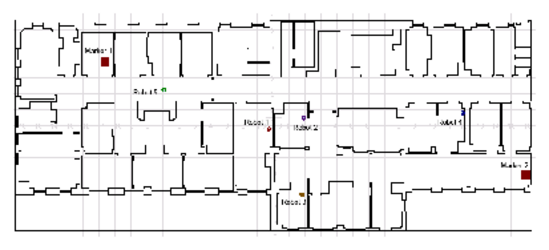Figure 5: Initial configuration 1 in a partial hospital floor plan ("hospital_section" in Stage). The map is 34x14 square meters. The robots (small circles are 15cm in diameter). The markers, shown as boxes, are resource locations. We aim to discover whether audio signaling can be used to improve performance of a robot system searching for the markers. To be feasible for real-world implementation in the short-term, we allow only very simple audio messages, representing single values from a pre-set range. This will be something similar to robots using DTMF codes, as used by a touch-tone telephone, to talk to each other. When a marker is seen and while it remains in view, the robot generates a DTMF tone identifying the marker. By continuing to announce the marker for a short period of time after the marker is no longer in view, it allows other robots to continue to receive location information, thereby increasing their chance of finding the markers. In our experiments this time is set to 10 seconds. In addition to receiving the marker number, other robots in the audible range will know audio volume and the direction from which the sound arrived. This is feasible in the real world: Valin [4] showed how microphone arrays can be used to detect the angle with high precision. However, a far more simple configuration is to have only two microphones and the direction can be simplified to two states: depending on the microphone placement, this could be front or rear, left or right. To use this information from the audio sensor, the messages received are stored in a queue with a time label. Each cell can now be scored based on the received messages and this score is added to the distance cost for scoring frontiers. These are the factors for scoring each cell based on one message:

• Difference of cell direction compared to message direction (-1.0 to 1.0)
• Message age (0.0 to 1.0)
• Message intensity (0.0 and 1.0)

In our implementation, for a cell c=(c_x,c_y), and the set M of messages, where each message is m=(m_data,m_θ,m_level,m_age), the cost function is:

f(c,M)=|c| + G − w ∏ m ∈ M  (Θ(mdir−cdir)Ω(mage) Φ(mlevel))

In which, |c|=√{c_x+c_y} is the cell distance from robot. G is a small Gaussian random with a mean of zero. w is a fixed weight. For 0 < x < 2π, Θ(x)=[(π−2x)/(π)], which is the direction difference factor. This is an approximation for Θ(x)=cos(x). Ω(m_age) is the message age factor and Ω(m_level) is the intensity factor. Messages are discarded from the queue after three minutes.

4.6  Sensor Choices

The swarm is made up of small two-wheeled robots, 15cm in diameter (a little larger than a CD) and the same height and a maximum speed of 30cm/second. The simulated sensors are configured to match the real devices as closely as possible given the limitations of Stage. For avoiding obstacles and to build a map of robot surroundings 8 infrared sensors with a range of 1.5m (similar to the real SHARP GP2D12 device) are used. To identify the markers showing the position of working areas, a camera and a simple blob finder with a range of 5 meters is assumed. Any fiducial-type sensor with the ability to guide the robot to a nearby line of sight object can be substituted. Two configurations of the simulated audio sensor were tested: omni-directional, i.e. giving high-resolution information about the direction to a sound source, and bi-directional, giving only 1 bit of direction data. The maximum audio receiving range was set to 15m.

5  Experiment

The environment map for this experiment is the "hospital section" map distributed with Stage, which is derived from a CAD drawing of a real hospital. It is a general office-like environment with rooms and corridors with a size of 34 by 14 meters. The map is large compared to the robot's size and sensor ranges (it is 227 ×93 times our 15 ×15cm robot size). A starting configuration is a list of starting position and angle for robots and the position of the two markers (working areas). A valid starting configuration is a starting configuration in which no object is placed over an obstacle and all markers are reachable. Ten different valid starting configurations are randomly generated. To illustrate, configuration 1 is shown in Figure 5. A job is defined as finding one marker and spending 30 seconds there working (loading/unloading) and then changing the goal to another marker. In each experiment the time for completing a total of 20 jobs by 5 robots is measured. So it is possible that different robots will complete different number of jobs. This means that if one robot becomes stuck somewhere, the other robots can continue to work.

6  Results

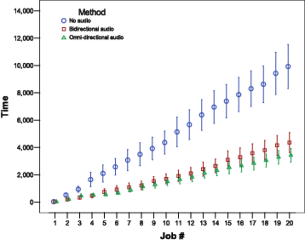
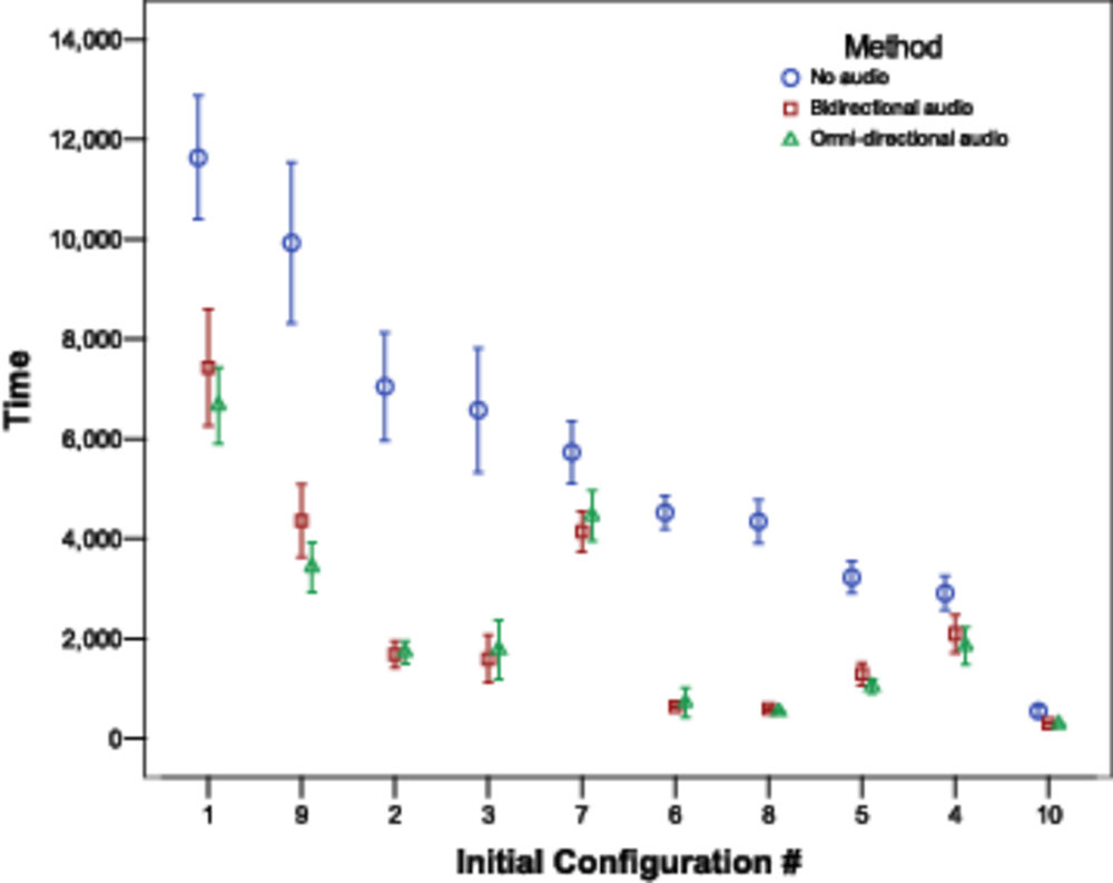
Figure 6: The mean and 95% confidence interval time (in seconds) to (a) finish each job in one of the initial configurations (configuration number 9) (b) finish all 20 jobs in all configurations. The configurations are reordered by the time of "no audio" method for the sake of clarity. We ran 20 experiments of 3 different methods over 10 different starting configurations, for a total of 600 simulation trials. Figure VI shows the mean and the 95% confidence interval of time to finish each job in one of the initial configurations (Configuration number 9). The chart shown in Figure VI shows the time to finish the total 20 jobs for all initial configurations. It can be seen that the most important factor in the total time to finish the job is the initial configuration and especially the position of the two working areas. In configuration 1, shown in Figure 5, the two markers are far apart, and the job-completion times seen in Figure VI for configuration 1 are large. However, in many configurations, differences in mean completion times between the three sensing methods are visible. To analyze these differences we ran t-tests between every pair of methods on each map to determine which pairs have significantly different means. We found that:

• For every map, there is a statistically significant difference between no audio and any method which uses attracting audio.
• Only two of the configurations using omni-directional sensors were statistically different from bi-directional ones
• Of these two, the differences were inconsistent.

From these results we can conclude that

1. using attracting audio can affect the performance significantly, and
2. as there is no statistical significant difference between an omni-directional and a bi-directional microphone, the use of a simple bi-directional can be recommended.

It should be noted that the size of the performance gain given by using audio is likely to be sensitive to the implementation parameters and environment properties. It also seems likely that the 1-bit audio direction sensor would not perform so well in less constrained environments.

7  Conclusion and Future Work

We have shown that using audio communication can increase the performance of a realistic group task significantly. This can be done even by using simple robots, each equipped with a speaker and two microphones as a bi-directional sensor, i.e. using one bit of audio signal direction information. The task and implementation presented here can be used as starting point for research in this field and there are many different aspects which could usefully be studied. There are several implementation parameters which can be changed, potentially affecting the overall performance of the system. Nonetheless, we believe that these simulation results are a useful predictor of the gross behavior of this system in the real world. Our future experiments will test this hypothesis. Due to its physical interaction with the robot's environment, audio promises to be a very interesting sensor modality. We plan to explore using frequency information in ambient and transmitted audio signals, for example to characterize locations by their "sound". As an example, our lab, offices and hallway have very different ambient sound and sound-reflection properties: each can be easily recognized by sound alone. This could be useful for localization. We also plan to explore the use of the audio in groups of agents, based on models of signaling behavior in birds and insects. Possible applications include resource management, territory formation, and task allocation. Another aspect of our work is to develop the robots, simulation and measurement tools for testing the algorithms. We also plan to further develop and test the audio propagation model, and make it available to the Player/Stage community.

References

[1]

J. Huang, T. Supaongprapa, I. Terakura, N. Ohnishi, and N. Sugie, "Mobile robot and sound localization," in Proc. IEEE Int. Conference on Intelligent Robots and Systems (IROS'97), September 1997.

[2]

E. Østergaard, M. J. Matari\'c, and G. S. Sukhatme, "Distributed multi-robot task allocation for emergency handling," in Proc. IEEE Int. Conference on Intelligent Robots and Systems (IROS'01), 2001, pp. 821 - 826.

[3]

M. Konishi, "Sound localization in owls," in Elsevier's Encyclopedia of Neuroscience, E. G. Adelman and B. H. Smith, Eds., 1999, pp. 1906-1908.

[4]

J. Valin, F. Michaud, J. Rouat, and D. Létourneau, "Robust sound source localization using a microphone array on a mobile robot," in Proc. IEEE Int. Conference on Intelligent Robots and Systems (IROS'03), 2003.

[5]

B. Gerkey, R. T. Vaughan, and A. Howard, "The Player/Stage project: Tools for multi-robot and distributed sensor systems," in Proc. Int. Conference on Advanced Robotics (ICAR'03), 2003, pp. 317-323.

[6]

R. T. Vaughan, K. Støy, G. S. Sukhatme, and M. J. Matari\'c, "Blazing a trail: Insect-inspired resource transportation by a robot team," in Int. Symposium on Distributed Autonomous Robotic Systems (DARS'02), 2000.

[7]

--, "Go ahead, make my day: robot conflict resolution by aggressive competition," in Proc. of Int. Conf. Simulation of Adaptive Behaviour, Paris, France, 2000.

[8]

2 plus 43 minus 4 C. Carollo, "Sound propagation in 3d environments," in Game Developers Conference (GDC'02), 2002. [Online]. Available: http://www.gamasutra.com/features/gdcarchive/2002/

[9]

M. de Berg, M. van Kreveld, M. Overmars, and O. Schwarzkopf, Computational Geometry: Algorithms and Applications.    NY: Springer, 1997.

[10]

2 plus 43 minus 4 E. W. Weisstein. (2002) Mathworld: Visibility graph. [Online]. Available: http://mathworld.wolfram.com/VisibilityGraph.html

[11]

E. W. Dijkstra, "A note on two problems in connexion with graphs," in Numerische Mathematik.    Mathematisch Centrum, Amsterdam, The Netherlands, 1959, vol. 1, pp. 269-271.

[12]

B. Yamauchi, "A frontier-based approach for autonomous exploration," in Proc. 1997 IEEE Int. Symposium on Computational Intelligence in Robotics and Automation, 1997.

[13]

P. Batavia and I. Nourbakhsh, "Path planning for the cye robot," in Proc. IEEE Int. Conference on Intelligent Robots and Systems (IROS'00), vol. 1, October 2000, pp. 15 - 20.

[14]

S. Moorehead, R. Simmons, and W. R. L. Whittaker, "Autonomous exploration using multiple sources of information," in Proc. IEEE Int. Conference on Robotics and Automation (ICRA'01), May 2001.